
"Edge AI" is used so loosely that it can mean almost anything with a chip in it. In industrial condition monitoring it means something specific: a small device, bolted to a machine, that turns a torrent of raw measurements into a handful of decisions without waiting for a data center. This article walks through how that works, stage by stage, and where the hard engineering problems sit.
Why the work moves to the device
Start with the data. A triaxial accelerometer sampling at 25.6 kHz with 16-bit resolution produces about 154 kilobytes per second. That is roughly 13 gigabytes a day from one sensor on one machine. A plant with a few hundred monitored assets would generate terabytes daily, nearly all of it describing machines behaving normally.
Shipping that volume is expensive on a wired network and often impossible on the cellular or low-power wireless links that industrial sites actually have. Latency is a second problem: a decision that depends on a round trip to a remote server is only as fast and as available as the link. The third reason is resilience. A monitoring system that goes blind whenever the network does is not much of a safety net.
So the first layers of interpretation run where the signal is. Cloud systems still matter, but their job changes from processing everything to learning from what the devices report.
The six stages
Most embedded condition-monitoring designs share the same skeleton, whatever the vendor calls the parts. The international standard for condition monitoring data processing, ISO 13374-1, describes a similar chain of functional blocks from data acquisition to advisory generation. On a device, it looks like this.

Acquire. Sensors are sampled at fixed rates chosen for the faults of interest. Bearing defects excite high frequencies, so vibration is sampled in the kilohertz range; temperature changes slowly and can be read once a second or less. Clean acquisition depends on the analog front end, the mounting and the sensor itself, and no amount of later processing recovers information that was never captured.
Condition. Raw samples are filtered to remove frequencies outside the band of interest, offset is removed, and data is cut into windows for analysis. This is also where the device checks data quality. A loose mount, a saturated sensor or electrical interference should be flagged as a measurement problem, not mistaken for a machine problem.
Extract. Windows are reduced to features that carry diagnostic meaning: overall RMS level, peak and crest factor, kurtosis, energy in frequency bands linked to known fault frequencies, and envelope spectra for bearing analysis. A spectrum of several thousand lines can be summarized in a few dozen numbers without losing what matters for most decisions.
Infer. Features are compared with a model of what normal looks like for this machine. That model might be statistical, such as a learned band for each feature at each operating condition, or a compact neural network trained to recognize patterns. The output is a score: how unusual is the present behavior, and does it resemble any known fault?
Decide. Most of the time the right decision is to stay quiet and log a summary. When a score crosses a threshold and stays there, the device raises a finding with its evidence attached. Persistence logic matters here. A single unusual window is often noise; a pattern that holds across hours is information.
Sync. Findings, daily summaries and occasional raw snapshots travel to the cloud when the link allows. Updated models travel back. The device keeps working when the link does not.
What gets thrown away
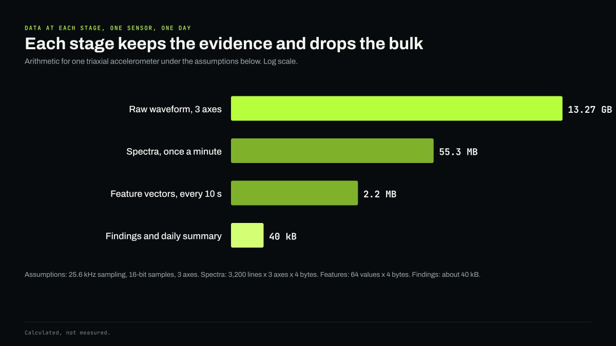
The art of edge design is deciding what is safe to discard. The chart below follows one sensor through the pipeline under stated assumptions. The raw waveform runs to about 13 gigabytes a day. Spectra stored once a minute come to around 55 megabytes. Feature vectors every ten seconds need about 2 megabytes. The findings and daily summary that actually reach a person fit in a few tens of kilobytes.
Throwing data away has a cost: you cannot reanalyze what you did not keep. Good designs hedge. They keep a rolling buffer of raw data on the device, so that when something interesting happens the waveform around the event can be uploaded for an engineer or a better model to examine later.
An example, step by step
A hypothetical case shows how the stages work together. A fan motor in an air handler develops a small defect on the outer race of its drive-end bearing. For the first few days, overall vibration barely changes, and a simple level alarm would see nothing. The extraction stage, however, tracks envelope energy at the bearing's outer-race defect frequency, which can be calculated from the bearing geometry and shaft speed. That feature begins to climb.
The inference stage compares the feature with the learned band for this motor at its current speed, and the score rises above its normal range. Persistence logic holds back for several hours to confirm the trend is real and not caused by a change in airflow. Once it has held, the device raises a finding: which bearing, which frequency, how far the feature has moved from baseline, and the motor's temperature trend for corroboration. It uploads a short raw waveform from its buffer so an analyst can check the spectrum. The whole exchange is a few hundred kilobytes, and in a case like this it can arrive well before the bearing becomes audible.
Fitting models into a small device
Running inference on a microcontroller used to be a research curiosity. It is now a mainstream engineering practice. Google's team described TensorFlow Lite Micro in 2020 as a framework for running neural networks on devices with only kilobytes of memory, and the MLPerf Tiny benchmark, published in 2021, includes an anomaly detection task based on machine sounds, which says something about how central industrial monitoring has become to the field.
The constraints are real all the same. Memory limits model size. Power limits how often the processor can run, especially on battery or harvested energy. Heat matters inside a sealed enclosure on a hot machine. The usual techniques are quantization, which stores model weights in 8-bit integers instead of 32-bit floats, careful feature engineering so the network has less to learn, and duty cycling, which wakes the full pipeline only when a cheap first-pass check suggests something has changed.
The hard part is not the model
The difficult problems in edge intelligence are less about the network architecture than about context. A machine's vibration depends on its speed and load. A model that does not know the operating state will mistake a change in duty for a change in health. Good edge systems track operating condition alongside condition indicators and compare like with like.
The second hard problem is lifecycle. Devices in the field need secure firmware and model updates, a way to roll back a bad update, and a record of which model produced which finding. Without that, nobody can audit a decision or improve the system with confidence.
The third is trust. An edge device makes judgments that people cannot see happening. Each finding has to carry its evidence: which feature moved, by how much, compared with what baseline. That is the difference between an alarm and an explanation.
A latency budget, worked through
It is worth putting rough numbers on the difference between analyzing on the device and sending raw data away. Take one second of three-axis vibration data sampled at 25.6 kilohertz with 16-bit samples: about 154 kilobytes.
| Step | On the device | Raw data sent to the cloud |
|---|---|---|
| Acquire one second of data | 1 second | 1 second |
| Move the data | None | About 1.2 seconds over a 1 megabit per second uplink, longer on a congested link |
| Transform and extract features | Tens of milliseconds on an efficient processor | Milliseconds on a server, after queueing |
| Compare with baseline and decide | Milliseconds | Milliseconds |
| Send the result | A few hundred bytes | Not needed |
| Data per day, continuous | Kilobytes to a few megabytes of findings | About 13 gigabytes |
The figures are illustrative, but the pattern holds. For a single decision, the time difference is modest, a second or two. The real difference is in volume and dependence. Streaming raw data from hundreds of machines would need network capacity that most sites do not have, and every decision would stop the moment the link dropped. Analysis on the device keeps both the data volume and the dependence small, which is why the edge carries the continuous work and the cloud carries the comparison and learning.
Where the cloud fits
None of this makes the cloud less important. It changes its role. The cloud is where findings from many machines are compared, where slow trends that span months are tracked, and where models are retrained on the evidence devices send back. A split architecture lets each layer do the work it is suited to: the device reacts to the machine in front of it, and the cloud learns across the fleet.
That division of labor sits at the center of edge AI for industrial systems as AFFERENT approaches it, and it shapes how NODE is being designed.


