
Every rotating machine shakes. A healthy motor, pump or fan shakes in a stable and repeatable way, set by its speed, its load and how it is built and mounted. When something starts to go wrong, the pattern changes. Vibration analysis is the discipline of measuring that pattern and working out what a change means.
It is one of the oldest and best understood tools in reliability engineering. Its limits have rarely been about physics. They have been about labor: collecting good data, turning it into something readable and having a trained analyst look at it often enough to matter. This guide walks through the chain from sensor to diagnosis, using real bearing data from a public test rig so the steps can be checked.
What a vibration sensor measures
The workhorse is the accelerometer, a small sensor bolted or bonded to a machine's housing, usually near a bearing. Piezoelectric accelerometers have long been the industrial standard because of their wide frequency range and low noise. MEMS accelerometers, built with the same fabrication methods as computer chips, are smaller and cheaper and have improved quickly, which is a large part of why continuous monitoring has become affordable.
Vibration can be expressed three ways, and each suits a different part of the spectrum.
- Displacement, in micrometers, emphasizes low frequencies. Proximity probes that measure shaft movement inside sleeve bearings on large turbines and compressors work in displacement.
- Velocity, in millimeters per second, gives a fairly even weighting across the range where most mechanical faults in general machinery appear. Overall severity limits for machines are usually written in velocity.
- Acceleration, in g, emphasizes high frequencies. Early bearing damage and gear problems show up here first.
How the sensor is attached matters as much as which sensor is chosen. A stud mount on a flat, clean surface passes high frequencies faithfully. A magnet is convenient for walk-around routes but loses some of the upper range. Placement matters too: readings are normally taken close to each bearing, in the radial directions and along the shaft axis, because different faults favor different directions.
Sampling decides what you can see
An accelerometer produces a continuous electrical signal, and the first irreversible decision is how to digitize it. The Nyquist criterion says the sampling rate must exceed twice the highest frequency of interest, and an anti-aliasing filter has to remove content above that limit before sampling, or high frequencies will fold back and masquerade as low ones. Many analyzers use a sampling rate of 2.56 times the analysis bandwidth, so a 10 kHz bandwidth implies 25.6 kHz sampling.
Record length matters just as much. The frequency resolution of a spectrum is the inverse of the time captured: one second of data gives 1 Hz resolution, ten seconds gives 0.1 Hz. Two faults with nearby frequencies, or a peak with closely spaced sidebands, can only be separated if the record is long enough. That is why a quick snapshot can miss what a patient measurement reveals.
From waveform to spectrum
The raw time waveform is useful for spotting impacts and transients, but it mixes everything together. The fast Fourier transform, or FFT, breaks the signal into its component frequencies, and that is where most diagnosis happens. Because so many fault mechanisms are tied to shaft speed, analysts read a spectrum in orders: 1x is running speed, 2x is twice running speed, and so on.
Decades of field experience have produced well-known patterns. They are starting points for an analyst, not verdicts.
| Condition | Where it tends to appear |
|---|---|
| Imbalance | A dominant peak at 1x in the radial direction, with few harmonics |
| Misalignment | High 1x in the axial direction for angular misalignment, high 2x radial for parallel offset |
| Mechanical looseness | A series of running-speed harmonics, sometimes with half-order peaks between them |
| Gear wear | Gear mesh frequency (number of teeth times shaft speed) and its harmonics, with sidebands spaced at shaft speed |
| Rolling bearing defects | Peaks at frequencies that are not whole multiples of running speed, often clearest after envelope analysis |
The last row is where most of the subtlety lives, because bearings are among the most common components in rotating equipment and their early damage is easy to miss in an ordinary spectrum.
Bearing frequencies follow from geometry
A rolling element bearing has four characteristic defect frequencies, and all of them can be calculated before the machine is ever switched on. They depend on the shaft speed, the number of rolling elements, the ball diameter, the pitch diameter and the contact angle. Each time a ball rolls over a spall on the outer race, it produces a small impact. Those impacts repeat at the ball pass frequency of the outer race, known as BPFO. Damage on the inner race repeats at BPFI, damage on a ball relates to the ball spin frequency (BSF), and cage problems show up at the fundamental train frequency (FTF).

The Case Western Reserve University Bearing Data Center, a public dataset that researchers have used for years to test diagnostic methods, publishes the geometry of its drive-end bearing, an SKF 6205-2RS deep groove ball bearing with nine balls. At the 1,796 rpm recorded for its no-load runs, the shaft turns at 29.93 Hz.
| Defect frequency | Multiple of shaft speed | At 1,796 rpm |
|---|---|---|
| Outer race (BPFO) | 3.585 | 107.3 Hz |
| Inner race (BPFI) | 5.415 | 162.1 Hz |
| Ball spin (BSF) | 2.357 | 70.5 Hz |
| Cage (FTF) | 0.398 | 11.9 Hz |
A ball defect often appears at twice BSF, because a damaged ball strikes both the inner and outer race on each spin. That is why the Case Western data tables list a rolling element multiple of 4.71.
Why bearings need envelope analysis
If the defect frequencies are known, it might seem enough to look for a peak at 107 Hz in the spectrum. In practice it usually is not. Each impact is very brief, so its energy is spread across a wide band and concentrated wherever the bearing housing and machine structure happen to resonate, typically several kilohertz. At 107 Hz itself, the fault contributes very little, and it sits underneath imbalance, misalignment and everything else the machine is doing.
Envelope analysis, also called demodulation, deals with this in three steps. First, filter the signal to a high-frequency band where the impacts excite resonances. Second, extract the envelope of that filtered signal, which traces the repeating bursts and discards the carrier. Third, take the spectrum of the envelope. The impact repetition rate, the defect frequency, now stands out clearly. Robert Randall and Jérôme Antoni's widely cited tutorial in Mechanical Systems and Signal Processing treats envelope analysis as the benchmark method for bearing diagnostics.
The figure below applies those steps to two Case Western recordings from the same motor at the same speed: one with a healthy bearing, one with a 0.18 mm defect seeded on the outer race.
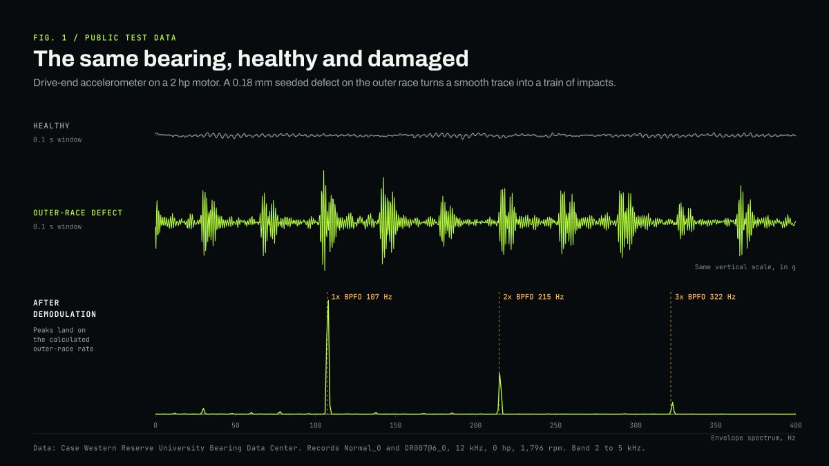
Even before any processing, the damaged bearing's waveform is visibly different: a train of impacts instead of a smooth trace. The envelope spectrum turns that difference into a diagnosis. Its largest peaks fall within a hertz or two of the calculated outer-race frequency and its second and third harmonics. A reliability engineer reading that plot knows which component is damaged and roughly where, without opening the machine.
How bad is it?
Finding a fault is half the job; judging its severity is the other half. The ISO 20816 series sets out a framework for evaluating machine vibration using four zones: A for newly commissioned machines, B for vibration acceptable for unrestricted long-term operation, C for levels that are unsatisfactory for long-term operation but tolerable for a limited period until action can be scheduled, and D for vibration severe enough to cause damage. The numeric boundaries depend on the machine type, size and how it is mounted, and the relevant part of the standard should be consulted for any specific machine.
Absolute limits are only part of the picture. Experienced analysts put as much weight on trend: how a machine's readings compare with its own history at similar speed and load, and how fast they are changing. A bearing moving steadily from zone B toward zone C over six weeks says more than a single reading taken once a quarter.
Where the bottleneck has been
None of the steps above are exotic. FFTs, envelope analysis, fault frequency calculation and trending are all well documented, and MathWorks publishes worked examples of bearing diagnosis using the same kind of data. The constraint has been coverage. Traditional programs send a technician on a route with a handheld collector, monthly or quarterly, and an analyst reviews the results. That works for critical machines. Most assets in a plant are never measured at all because the labor costs more than the machine.
Continuous sensing changes the economics, but only if interpretation comes with it. A sensor that streams waveforms to a server just moves the analyst's workload somewhere else. The useful version runs the analysis beside the sensor, learns what normal looks like for that particular machine at its usual speeds and loads, and reports a finding with its evidence when the pattern shifts. The harder engineering problems are context and confidence: separating a real fault from a change in load or speed, and knowing when not to raise an alarm.
The math behind vibration analysis isn't new. The opportunity is to make that intelligence more continuous, more accessible and useful across far more machines than traditional inspection can realistically cover.

Why vibration carries so much information in the first place is the subject of Why Failure Has a Signature. The sensing modalities AFFERENT is designing around, vibration among them, are described on our multimodal industrial sensing page, and the hardware intended for heavy rotating equipment is NODE Industrial.
Vibration analysis has never lacked rigor. It has lacked reach. Bringing the methods described here to the thousands of motors, pumps and fans that have never had an analyst look at them is the practical work of machine health intelligence, and most of it comes down to doing well-understood math reliably, at the edge, every day.
Sources
- Case Western Reserve University Bearing Data Center: bearing information
- Case Western Reserve University Bearing Data Center: 12k drive end bearing fault data
- Case Western Reserve University Bearing Data Center: normal baseline data
- Randall and Antoni: Rolling element bearing diagnostics, a tutorial (Mechanical Systems and Signal Processing, 2011)
- ISO 20816-3:2022 Mechanical vibration, industrial machinery above 15 kW
- NTN: Formulas to calculate bearing frequencies
- MathWorks: Rolling element bearing fault diagnosis
- Fluke: Diagnosing imbalance, misalignment, looseness and bearing wear


