
Every predictive maintenance program eventually meets the same test. An alert arrives for a machine that a technician knows well. Someone walks out, listens, measures, looks, and finds nothing wrong. It happens again the following week on a different machine. By the third or fourth time, the alerts are being read with a sigh, and the program has started to fail, even if the software is working exactly as designed.
False positives get less attention than missed faults because they rarely cause a dramatic event. They cause something slower: a loss of trust that turns a monitoring system into background noise. This article explains why false alarms are so common even with good models, works through the arithmetic with real numbers, and sets out the design choices that keep them under control.
The arithmetic of rare events
Developing faults are rare. In a well run plant, most machines are healthy most of the time. That simple fact has a large and unintuitive effect on how alerts behave.
Take a fleet monitored for 1,000 machine-months, which is roughly a year of watching 83 machines. Suppose 10 of those machine-months contain a real developing fault that a good system ought to catch. Now suppose the detector is good by most standards: it catches 80 percent of real faults, and it stays quiet on 95 percent of healthy machine-months.
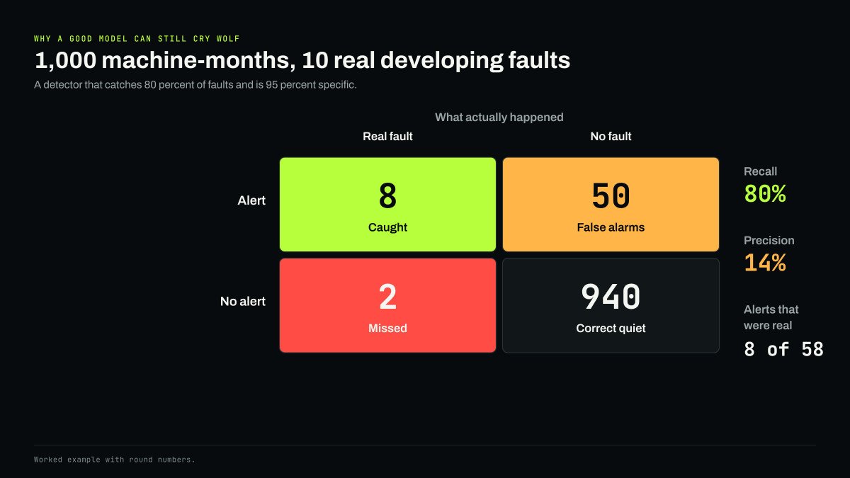
The detector catches 8 of the 10 faults and misses 2. Of the 990 healthy machine-months, it correctly stays quiet on 940 and raises an alert on 50. The maintenance team receives 58 alerts in total, and 8 of them are real. Precision, the share of alerts that are real, is about 14 percent.
Nothing is wrong with the model in this example. It is the base rate. When healthy cases outnumber faulty ones by 99 to 1, even a small false alarm rate on the healthy side produces more alerts than the real faults do. Statisticians call the mistake of ignoring this the base rate fallacy, and it catches out experienced engineers as easily as anyone.
Specificity matters more than it looks
The way out is not obvious from headline accuracy figures. A detector that is 95 percent specific sounds almost as good as one that is 99.9 percent specific. On rare events they behave completely differently. The table holds recall at 80 percent and the fault rate at 1 percent, and changes only specificity.
| Specificity | False alarms per 1,000 machine-months | Real alerts | Precision |
|---|---|---|---|
| 95 percent | about 50 | 8 | 14 percent |
| 99 percent | about 10 | 8 | 45 percent |
| 99.5 percent | about 5 | 8 | 62 percent |
| 99.9 percent | about 1 | 8 | 89 percent |
Moving from 95 to 99.9 percent specificity turns a system where six alerts in seven are false into one where nearly nine in ten are real. That last few percent is where most of the engineering effort in a good monitoring system goes.
The same point applies when evaluating systems. Takaya Saito and Marc Rehmsmeier showed in a 2015 PLOS ONE study that on imbalanced data, ROC curves can make a classifier look much better than it will feel in use, and that precision and recall plots give a more informative picture. A vendor quoting a high area under the ROC curve on fault data has told you something, but not the thing a maintenance team will experience. Ask for precision at the operating threshold, on data with a realistic fault rate.
Choosing the threshold is choosing a cost
Every detector has a dial. Turn the alert threshold down and it catches more real faults but raises more false alarms. Turn it up and the false alarms fall away, along with some of the real faults.

The right setting depends on what each kind of error costs. Suppose a false alarm costs $400, the time for a technician to visit and check a machine. Suppose a missed fault costs $20,000, the difference between a planned repair and an unplanned failure with secondary damage. Using the same 1,000 machine-months and 10 real faults, three thresholds give these results.
| Threshold | Faults caught | Missed | False alarms | Cost of misses | Cost of false alarms | Total |
|---|---|---|---|---|---|---|
| Low | 9 | 1 | 104 | $20,000 | $41,600 | $61,600 |
| Middle | 8 | 2 | 50 | $40,000 | $20,000 | $60,000 |
| High | 6 | 4 | 10 | $80,000 | $4,000 | $84,000 |
In this example, the low and middle settings cost about the same, and the high setting costs the most because missed faults are expensive. Change the inputs and the answer moves. If the machine is a critical pump whose failure costs $200,000, the low threshold wins easily. If a false alarm means sending a crew three hours to a remote site at $3,000 a visit, the high threshold starts to look sensible.
One cost that matters most over time is missing from the table: what 104 false alarms a year do to the people receiving them. The financial model treats each false alarm as $400. The team treats the hundredth one as a reason to stop looking.
What the control room already learned
Process industries went through this decades ago with control room alarms. Poorly designed alarm systems produced so many alerts that operators could not respond to them meaningfully, and investigations of several serious incidents found important alarms buried in floods of unimportant ones. The response was a discipline of alarm management, codified in the ISA-18.2 standard and in EEMUA Publication 191.
The targets give a sense of scale. A summary of ISA-18.2 suggested values published by ISA Ireland puts the acceptable range at 150 to 300 annunciated alarms per operator position per day, roughly 6 to 12 an hour, with about 80 percent low priority, 15 percent medium and 5 percent high, and zero chattering alarms. Those numbers are for operators watching a live process, not maintenance planners. But the principle carries over directly: every alert must be actionable, priorities must mean something, and an alert that fires repeatedly without anyone acting is a defect in the system, not a feature.
Where false positives come from
In machine monitoring, false alarms have a small number of common sources, and each has a known remedy.
Operating changes. A pump that moves to a new duty point, a fan that changes speed or a compressor that starts loading differently can look abnormal to a model trained on a narrower range. The remedy is to learn normal behavior across operating states and to give the model context about speed, load and setpoints.
Environment. Temperatures follow the weather. Vibration can change with foundation conditions and nearby equipment. Models that account for ambient conditions avoid flagging every heat wave.
Sensor and installation faults. A loose mount, a damaged cable or electrical noise from a drive produces data that look alarming and say nothing about the machine. Monitoring systems need to check the health of their own sensors and say so when the data cannot be trusted.
Maintenance events. Regreasing a bearing, realigning a coupling or replacing a belt changes a machine's signature, usually for the better. A system that knows when work was done can treat the change as expected.
Single-signal decisions. One signal crossing a line is weak evidence. Several independent signals telling a consistent story is strong evidence. Requiring corroboration across vibration, acoustic, thermal and electrical data, and requiring a change to persist across several measurement windows, removes a large share of false alarms at little cost in sensitivity.
That last point is often the most effective single change. Distinguishing a real developing fault from a passing anomaly is the subject of our explainer on anomalies and failures, and persistence plus corroboration is the practical way to make that distinction automatically.
Close the loop
The most valuable data a monitoring program can collect is also the most often neglected: what happened after each alert. Was a fault found? Which one? Was it a sensor problem, an operating change, or nothing at all? Without that record, nobody can measure precision, thresholds cannot be tuned against reality, and the system never gets better.
Programs that do this well make it nearly effortless. The technician who checks the machine records the outcome in a few taps, ideally in the work order system they already use. Over months, those outcomes become the labeled data that let models learn which patterns precede real faults on that site's machines, and which are harmless.
Measures worth tracking
- Alert precision: the share of alerts that led to a confirmed finding, tracked monthly.
- Alerts per asset per month: a rising number on one machine usually means a model or sensor problem.
- Outcome coverage: the share of alerts with a recorded result. Below about 80 percent, precision figures are guesses.
- Repeat alerts: the same alert on the same machine with no action taken. Each one is a candidate for retuning.
- Missed faults: failures that occurred on monitored machines without a prior alert, each one reviewed.
The goal is not zero false alarms. A system tuned to never raise a false alarm will miss faults it should have caught. The goal is a level of precision that the people receiving alerts can trust, sustained over time. That is what reliable machine anomaly detection means in practice, and it is what separates programs that last from the ones that are switched off after a year.
Sources
- Saito and Rehmsmeier, The Precision-Recall Plot Is More Informative than the ROC Plot When Evaluating Binary Classifiers on Imbalanced Datasets, PLOS ONE (2015)
- ISA Ireland: Alarm System Performance Metrics, ISA-18.2 suggested targets (2016)
- ISA-18 series: Management of Alarm Systems for the Process Industries
- EEMUA Publication 191: Alarm systems, a guide to design, management and procurement


